Interactive online version:

Part III: Post analysis (Python/Jupyter/Colab)

This tutorial is a Jupyter notebook that illustrates how to load & open output files from Tapqir analysis. To work with the live version of the notebook run it in Google Colab using the link above.

Set up the environment

• Connect Google Drive to be able to save the analysis output (to view Files & Folders click on a Folder icon on the left):

# Run this cell to connect to Google Drive
from google.colab import drive

drive.mount("/content/drive")

Mounted at /content/drive

• Run the cell below to install tapqir (takes about a minute):

!pip install --quiet tapqir > install.log

Load data & analysis results

Extracted AOI images are stored in a data.tpqr file; analysis results are stored in a cosmos-channel0-params.tpqr and cosmos-channel0-summary.csv files. We will import cosmos model from tapqir, create its instance, and then call .loadmethod to load these files:

# import cosmos model
from tapqir.models import Cosmos

# create a cosmos model instance
model = Cosmos()
# load analysis results from the working directory
model.load(path="/content/drive/MyDrive/tutorial", data_only=False)

AOI images

# data can be accessed through .data attribute
model.data

CosmosDataset: Rpb1SNAP549
  images           tensor(N=331 on-target AOIs, Nc=526 off-target AOIs, F=790 frames, C=1 channels, P=14 pixels, P=14 pixels)
  x                tensor(N=331 on-target AOIs, Nc=526 off-target AOIs, F=790 frames, C=1 channels)
  y                tensor(N=331 on-target AOIs, Nc=526 off-target AOIs, F=790 frames, C=1 channels)

  offset.samples   tensor([ 90,  91,  92,  93,  94,  95,  96,  97,  98,  99, 100, 101, 102, 103,
                          104, 105, 106, 107, 108, 109, 110, 111, 112, 113, 114, 115, 116],
                         dtype=torch.int32)
        .weights   tensor([2.8129e-06, 6.7511e-05, 4.1210e-04, 1.7932e-03, 7.1871e-03, 2.1366e-02,
                          4.7677e-02, 9.0093e-02, 1.3192e-01, 1.6421e-01, 1.5248e-01, 1.0433e-01,
                          7.7949e-02, 5.2655e-02, 3.5667e-02, 2.2335e-02, 1.9520e-02, 1.6328e-02,
                          1.2553e-02, 8.6892e-03, 7.2546e-03, 5.8228e-03, 4.4402e-03, 3.1153e-03,
                          2.5893e-03, 2.3038e-03, 7.2433e-03], dtype=torch.float32)

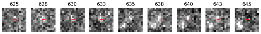
Data is stored as a CosmosDataset object that has a title (Rpb1SNAP549), images attribute for AOI images (torch.Tensor object with (N+Nc, F, C, P, P) shape), x attribute for target locations on the x-axis (torch.Tensor with (N+Nc, F, C) shape), and y attribute for target locations on the y-axis (torch.Tensor with (N+Nc, F, C) shape), and offset attribute for camera offset data.

As an example let’s plot frames 625, 628, 630, 633, 635, 638, 640, 643, 645 from AOI 163 and also show target locations (red + sign).

# import matplotlib for plotting
import matplotlib.pyplot as plt

fig = plt.figure(figsize=(15, 1.5))
n = 163  # AOI
c = 0  # color channel
frames = [625, 628, 630, 633, 635, 638, 640, 643, 645]

for i, f in enumerate(frames):
    ax = fig.add_subplot(1, 9, i + 1)
    ax.imshow(model.data.images[n, f, c].numpy(), vmin=340, vmax=635, cmap="gray")
    ax.scatter(
        model.data.x[n, f, c].item(),
        model.data.y[n, f, c].item(),
        c="r",
        s=100,
        marker="+",
    )
    ax.set_title(f, fontsize=16)
    ax.axis("off")

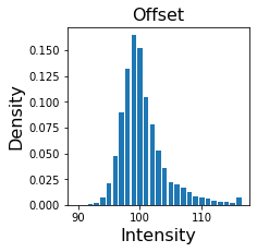
Offset distribution

offset is an OffsetData object that has samples attribute for camera offset values and weights attribute for their probabilities (together they define and Empirical distribution for the offset signal). Let’s plot it.

plt.figure(figsize=(3, 3))
plt.bar(model.data.offset.samples, model.data.offset.weights)
plt.title("Offset", fontsize=16)
plt.ylabel("Density", fontsize=16)
plt.xlabel("Intensity", fontsize=16)
plt.show()

Parameters

Model parameters with 95% CI (credible interval) are stored in cosmos-params.tpqr file (nested dictionary of torch.Tensors). It can be accessed using a .params attribute:

# list all parameters
model.params.keys()

dict_keys(['gain', 'proximity', 'lamda', 'pi', 'Keq', 'height', 'width', 'x', 'y', 'background', 'm_probs', 'theta_probs', 'z_probs', 'z_map', 'p_specific', 'time1', 'ttb', 'h_specific', 'chi2'])

• gain - \(g\) camera gain

• proximity - \(\sigma^{xy}\) proximity

• lamda - \(\lambda\) off-target binding rate

• pi - \(\pi\) average on-target binding probability

• Keq - equilibrium constant calculated as \(\frac{\pi}{1-\pi}\)

• z_probs - \(p(z=1|D)\) probability of there being any target-specific spot in an AOI image

• p_specific - \(p(\mathsf{specific})\) probability of there being any target-specific spot in an AOI image

• z_map - most likely value (0 or 1) for target-specific spot presence (obtained from \(p(\mathsf{specific})\) using 0.5 cutoff)

• theta_probs - \(p(\theta=k|D)\) target-specific spot index probabilities

• m_probs - \(p(m=1|D)\) spot presence probabilities

• height - \(h\) spot intensity

• width - \(w\) spot width

• x - \(x\) spot position on x-axis

• y - \(y\) spot position on y-axis

• background - \(b\) background intensity

For example, let’s look at gain \(g\):

model.params["gain"]

{'LL': tensor(6.7341), 'UL': tensor(6.7392), 'Mean': tensor(6.7366)}

It is a dictionary with the values of the mean (Mean), 95% credible interval lower-limit (LL) and upper-limit (UL).

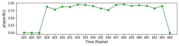
Let’s plot \(p(\mathsf{specific})\) for AOI 163 and frames from 625 to 645:

n = 163
f1, f2 = 625, 645

plt.figure(figsize=(10, 2))
plt.plot(range(f1, f2), model.params["z_probs"][n, f1:f2], "o-", color="C2")
plt.ylabel(r"$p(\mathsf{specific})$", fontsize=12)
plt.xlabel("Time (frame)", fontsize=12)
plt.xticks(range(f1, f2))
plt.show()

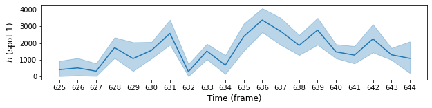
To plot credible intervals we can use pyplot’s fill_between method. Here is the plot of intensity \(h\) for spot 1 in the same range of frames:

k = 0  # spot 1
n = 163  # AOI
f1, f2 = 625, 645  # frame range

plt.figure(figsize=(10, 2))
plt.plot(range(f1, f2), model.params["height"]["Mean"][k, n, f1:f2], "-", color="C0")
plt.fill_between(
    range(f1, f2),
    model.params["height"]["LL"][k, n, f1:f2],
    model.params["height"]["UL"][k, n, f1:f2],
    color="C0",
    alpha=0.3,
)
plt.ylabel(r"$h$ (spot 1)", fontsize=12)
plt.xlabel("Time (frame)", fontsize=12)
plt.xticks(range(f1, f2))
plt.show()

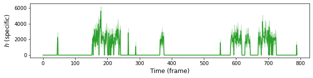
Here we plot ntensities of target-specifics. Target-specific spot is selected from two spots using 0.5 probability cut-off.

n = 163  # AOI
theta_mask = model.params["theta_probs"][:, n] > 0.5
height_mean = (model.params["height"]["Mean"][:, n] * theta_mask).sum(0)
height_ll = (model.params["height"]["LL"][:, n] * theta_mask).sum(0)
height_ul = (model.params["height"]["UL"][:, n] * theta_mask).sum(0)

plt.figure(figsize=(10, 2))
plt.plot(range(0, model.data.F), height_mean, "-", color="C2")
plt.fill_between(
    range(0, model.data.F),
    height_ll,
    height_ul,
    color="C2",
    alpha=0.3,
)
plt.ylabel(r"$h$ (specific)", fontsize=12)
plt.xlabel("Time (frame)", fontsize=12)
plt.show()

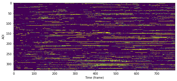
Probabilistic rastergram

We can plot \(p(\mathsf{specific})\) as a probabilistic rastergram.

import matplotlib as mpl

plt.figure(figsize=(10, 5))
plt.imshow(
    model.params["z_probs"][: model.data.N],
    norm=mpl.colors.Normalize(vmin=0, vmax=1),
    aspect="equal",
    interpolation="none",
)
plt.ylabel("AOI")
plt.xlabel("Time (frame)")
plt.show()

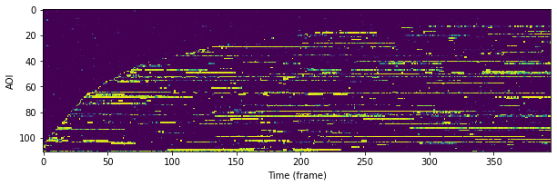
Probabilistic rastergram with AOIs ordered by time-to-first binding:

from tapqir.utils.imscroll import time_to_first_binding

# sorted on-target
ttfb = time_to_first_binding(model.params["z_map"][: model.data.N])
# sort ttfb
sdx = torch.argsort(ttfb, descending=True)

plt.figure(figsize=(10, 5))
norm = mpl.colors.Normalize(vmin=0, vmax=1)
im = plt.imshow(
    model.params["z_probs"][: model.data.N][sdx][::3, ::2],
    norm=norm,
    aspect="equal",
    interpolation="none",
)
plt.xlabel("Time (frame)")
plt.ylabel("AOI")
cbar = plt.colorbar(im, ax=ax, aspect=8, shrink=0.9)
cbar.set_label(label=r"$p(\mathsf{specific})$")

Global parameters

summary attribute (loaded from the cosmos-channel0-summary.csv file) contains values of global parameters (for easy access).

model.summary

	Mean	95% LL	95% UL
gain	6.736577	6.734092	6.739194
proximity	0.607815	0.604436	0.611418
lamda	0.288701	0.287115	0.290384
pi	0.092999	0.092036	0.093988
Keq	0.102533	0.101366	0.103738
SNR	1.606830	NaN	NaN