Part II: Tapqir analysis (Linux/Windows)#
In this tutorial we will use a linux computer to analyze the Data set A in Ordabayev et al., 2022. The data are taken from Rosen et al., 2020 and have already been preprocesssed using imscroll (Friedman et al., 2015).
Set up the environment#
Download input data#
These data were acquired with Glimpse and pre-processed with the imscroll program (Friedman et al., 2015). Change directory to user’s home directory:
$ cd ~
Download data files using wget:
$ wget https://zenodo.org/record/5659927/files/DatasetA_glimpse.zip
Unzip and then delete the zip file:
$ unzip DatasetA_glimpse.zip && rm DatasetA_glimpse.zip
The raw input data placed in /home/{your_username}/DatasetA_glimpse are:
garosen00267- folder containing image data in glimpse format and header filesgreen_DNA_locations.dat- aoiinfo file designating target molecule (DNA) locations in the binder channelgreen_nonDNA_locations.dat- aoiinfo file designating off-target (nonDNA) locations in the binder channelgreen_driftlist.dat- driftlist file recording the stage movement that took place during the experiment
To start the analysis create an empty folder (here named tutorial) which will be the working directory:
$ mkdir ~/tutorial
Start the program#
To start the program run:
$ tapqir-gui
which will open a browser window to display the Tapqir GUI:

Select working directory#
Click the Select button to set the working directory to /home/{your_username}/tutorial:
Setting working directory creates a .tapqir sub-folder that will store internal files
such as config.yaml configuration file, loginfo logging file, and model checkpoints.
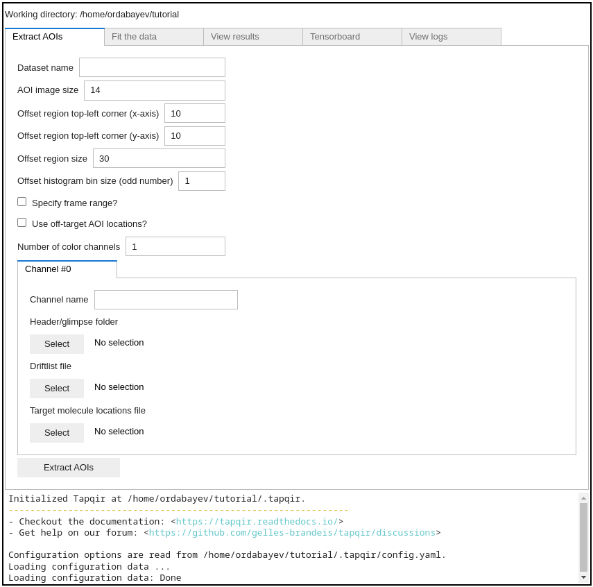
Extract AOIs#
To extract AOIs specify the following options in the Extract AOIs tab:
A dataset name:
Rpb1SNAP549(an arbitrary name)Size of AOI images: we recommend using
14pixelsStarting and ending frame numbers to be included in the analysis (
1and790). If starting and ending frames are not specified then the full range of frames from the driftlist file will be analyzed.The number of color channels:
1(this data set has only one color channel available)Use off-target AOI locations?:
True(we recommended including off-target AOI locations in the analysis)
And specify the locations of input files for each color channel (only one color channel in this example):
Channel name:
SNAP549(an arbitrary name)Header/glimpse folder:
/home/{your_username}/DatasetA_glimpse/garosen00267Driftlist file:
/home/{your_username}/DatasetA_glimpse/green_driftlist.datTarget molecule locations file:
/home/{your_username}/DatasetA_glimpse/green_DNA_locations.datOff-target control locations file:
/home/{your_username}/DatasetA_glimpse/green_nonDNA_locations.dat
See Advanced settings below for details on adjusting offset parameters.
Note
About indexing. In Python indexing starts with 0. We stick to this convention and index AOIs, frames, color channels,
and pixels starting with 0. Note, however, that for starting and ending frame numbers we used 1 and 790 which are according to
Matlab indexing convention (in Matlab indexing starts with 1) since driftlist file was produced using a Matlab script.
Next, click Extract AOIs button:
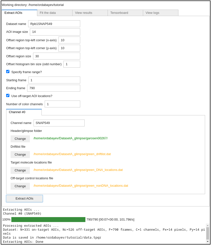
Great! The program has outputted a data.tpqr file containing extracted AOI images (N=331 target and Nc=526 off-target
control locations):
$ ls ~/tutorial

data.tpqr            offset-distribution.png  offtarget-channel0.png
offset-channel0.png  offset-medians.png       ontarget-channel0.png
Additionally, the program has saved
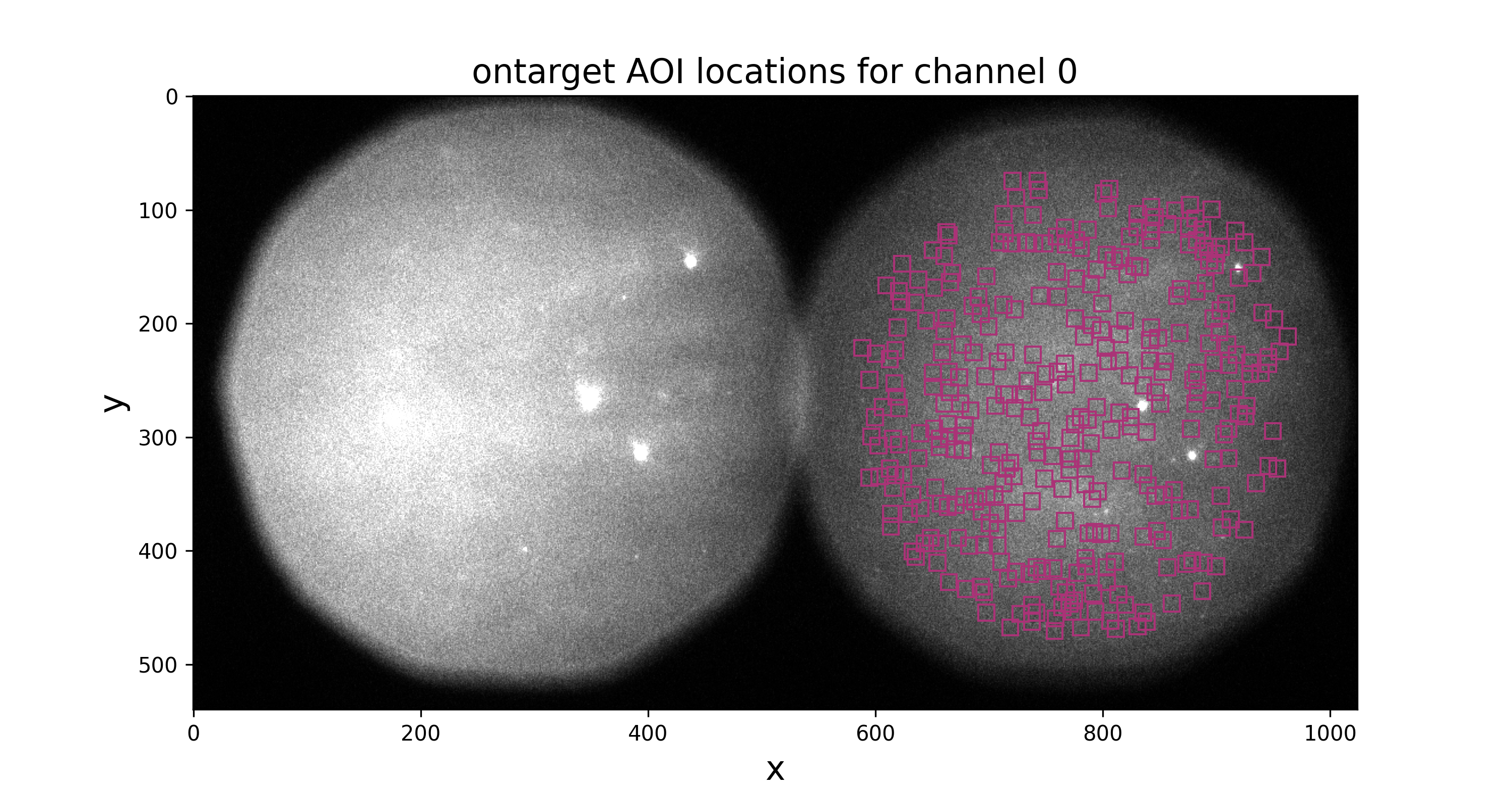
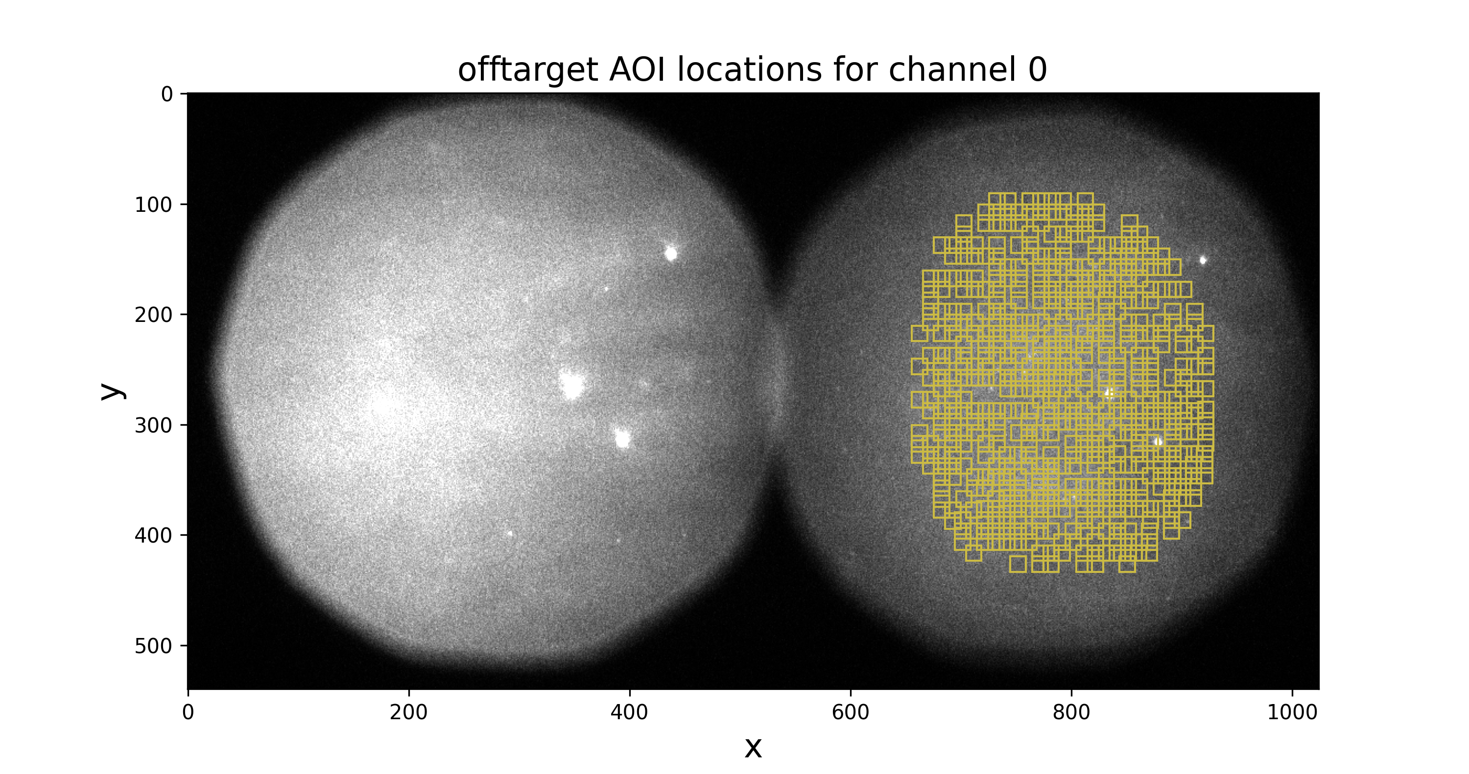
Image files (
ontarget-channel0.pngandofftarget-channel0.png) displaying locations of on-target and off-target AOIs in the first frame. You should inspect these images to make sure that AOIs are inside the field of view:
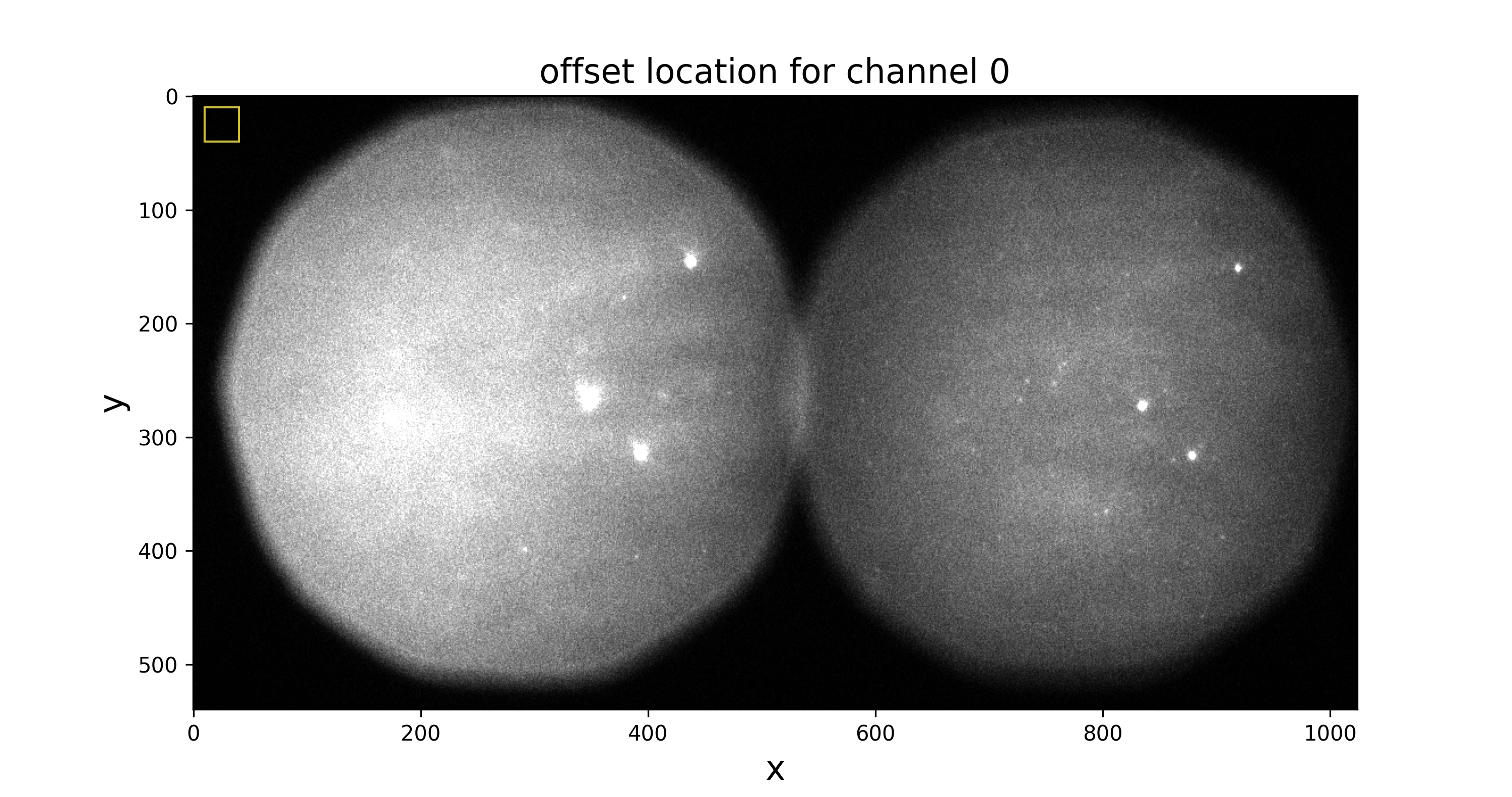
You should also look at
offset-channel0.pngto check that offset data is taken from a region outside the field of view:
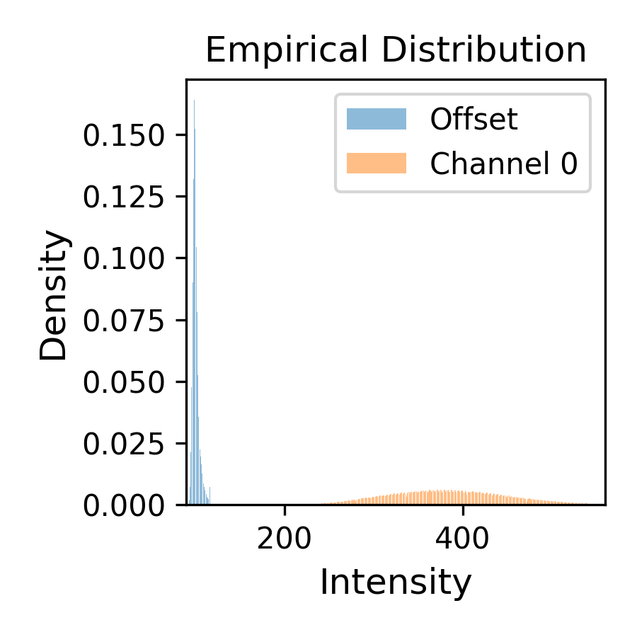
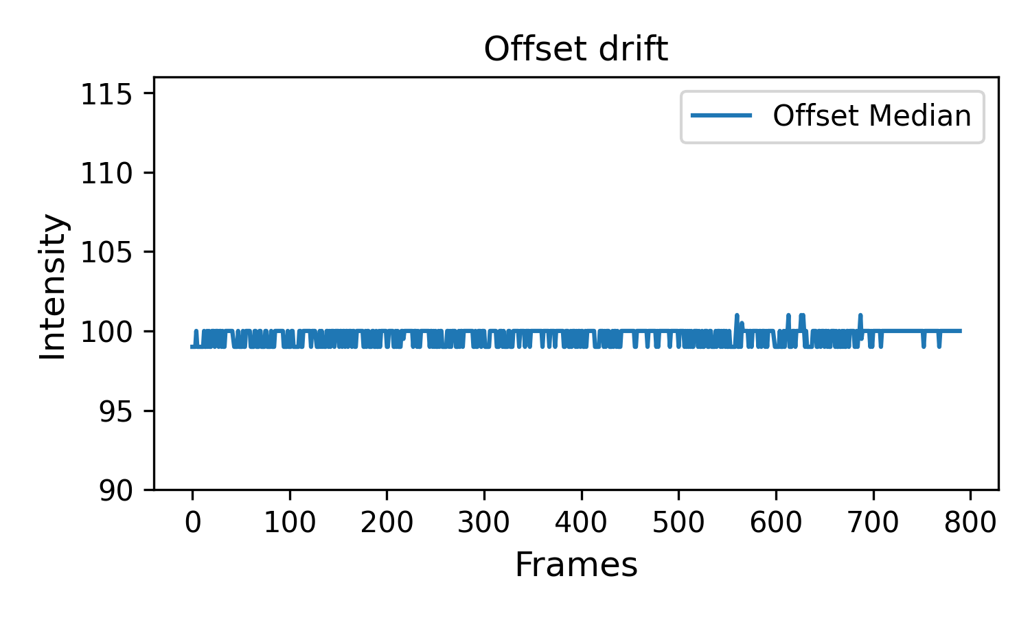
The other two files show the intensity histograms (
offset-distribution.png) and the offset median time record (offset-medians.png) (offset distribution shouldn’t drift over time):
Fit the data#
Now the data is ready for fitting. Options that we will select:
Model - the default single-color time-independent
cosmosmodel (Ordabayev et al., 2022).Color channel number - first chanel (
0) (there is only one color channel in this data)Run computations on GPU: yes (
True).AOI batch size - use default (
10).Frame batch size - use default (
512).Learning rate - use default (
0.005).Number of iterations - use default (
0)
See Advanced settings below for details on adjusting prior parameters.
Note
About batch size. Batch sizes should impact training time and memory consumption. Ideally,
it should not affect the final result. Batch sizes can be optimized for a particular GPU hardware by
trying different batch size values and comparing training time/memory usage
(nvidia-smi shell command shows Memory-Usage and GPU-Util values).
Next, press Fit the data button:
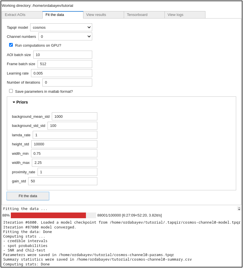
The program will automatically save a checkpoint every 200 iterations (checkpoint is saved at .tapqir/cosmos_model.tpqr).
The program can be stopped at any time by clicking in the terminal window and pressing Ctrl-C. To restart the program again re-run
tapqir-gui command and the program will resume from the last saved checkpoint.
After fitting is finished, the program computes 95% credible intervals (CI) of model parameters and saves the parameters and CIs in
cosmos_params.tqpr, cosmos_params.mat (if Matlab format is selected), and cosmos_summary.csv files.
If you get an error message saying that there is a memory overflow you can decrease either frame batch size (e.g., to 128 or 256)
or AOI batch size (e.g., to 5).
Tensorboard#
At every checkpoint the values of global variational parameters (-ELBO, gain_loc, proximity_loc,
pi_mean, lamda_loc) are recorded. Fitting progress can be inspected while fitting is taking place or afterwards with the tensorboard program
displayed in the Tensorboard tab, which shows the parameters values as a function of iteration number:
Note
On WSL the Tensorboard tab does not work. To view tensorboard open a new terminal, activate the environment:
$ conda activate tapqir-env
run tensorboard:
$ tensorboard --logdir=<your working directory>
and then open localhost port (typically http://localhost:6006) in a browser window. To quit tensorboard press Ctrl-C.
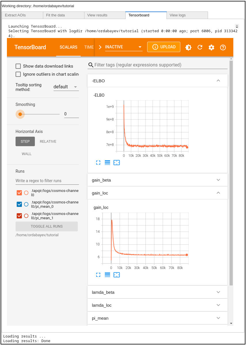
Tip
Set smoothing to 0 (in the left panel) and use refresh button at the top right to refresh plots.
Plateaued plots of -ELBO, gain_loc, proximity_loc, pi_mean, and lamda_loc signify convergence.
Note
About number of iterations. Fitting the data requires many iterations (about 50,000-100,000) until parameters converge. Setting the number of iterations to 0 will run the program till Tapqir’s custom convergence criterion is satisfied. We recommend to set it to 0 (default) and then run for additional number of iterations if required.
View results#
After fitting is done open View results tab to visualize analysis results. Click on Load results button which will display parameter values
from the cosmos_params.tpqr file:
Note
cosmos_params.tpqr file is generated after fitting has completed (either when specified number of iterations has finished or
the model has converged).
Note
If Show FOV images is checked then the image of the entire field of view will be displayed at the bottom. Note, however,
that raw glimpse files as specified at AOI extraction step need to be present on the local disk.
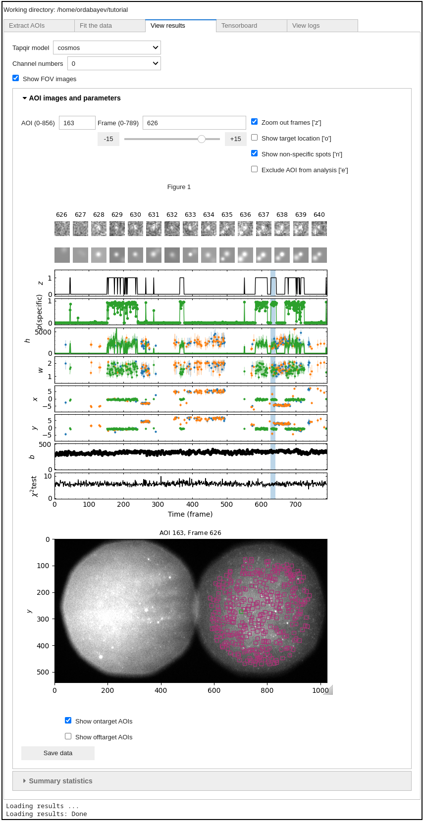
In the display panel:
the top row shows raw images and the second row shows best fit images
target-specific spot presence probability
p(specific)and its most likely valuezvalues (mean and 95% CI) of
h,w,x,y, andbparameters for target-specific spot (green) and target-nonspecific spots (spot 1 is blue and spot 2 is orange; remember that spot numbering is arbitrary)chi-squared test of how well the model fits each particular image (higher number means worse fit)
The AOI number can be changed using the box widget or Down, Up arrow keys or j, k keys
(hover the mouse over the View results tab for keys to work).
Frame range can be toggled to zoom out to entire frame range by clicking on the Zoom out frames checkbox
or using the z key. When zoomed out the range of frames corresponding to AOI images is highlighted in blue.
The frame range can be changed by using the slider widget at the top or Left, Right arrow keys or h, l
keys or by left-clicking on the plot.
Advanced settings#
Offset#
Offset data region (yellow square) can be edited using three variables:
offset_x: left corner of the square (default is 10 pixels)offset_y: top corner of the square (default is 10 pixels)offset_P: size of the square (default is 30 pixels)
Bin size for the offset intensity histogram by default is 1. The bin size can be increased (try 3 or 5; odd number) to make the histogram sparser which will speed up fitting.
bin_size: offset intensity histogram bin size (default is 1)
Prior distributions#
Parameters of prior distirbutions (Eqs. 6a, 6b, 11, 12, 13, 15, and 16 in Ordabayev et al., 2022):
background_mean_std(default 1000): standard deviation of the HalfNormal distribution in Eq. 6abackground_std_std(default 100): standard deviation of the HalfNormal distribution in Eq. 6blamda_rate(default 1): rate parameter of the Exponential distribution in Eq. 11heiht_std(default 10,000): standard deviation of the HalfNormal distribution in Eq. 12width_min(default 0.75): minimum value of Uniform distribution in Eq. 13width_max(default 2.25): maximum value of Uniform distribution in Eq. 13proximity_rate(default 1): rate parameter of the Exponential distribution in Eq. 15gain_std(default 50): standard deviation of the HalfNormal distribution in Eq. 16